Cellular Automata: A Primer

Automata are, fundamentally, computing media. Their origins date to Turing's work on computable numbers in the 1930s. Examples from the computer sciences include finite state machines, Turing machines, and artificial neural networks. These basic computing automata may be characterized as follows:

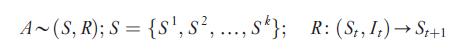
where A represents an automaton, characterized by states S and a transition rule R. The transition rule functions to manage changes in states S from time t to time t+1, given input of other state information from outside the automaton at time t. The transition rule becomes the medium of exchange and states become the raw material when many such automata are designed to co interact. Automata of this form resemble Markov models (which deal with serial autocorrelation in temporal transition) and raster models (which deal with layering of statespace).

The cellular automaton (CA) adds an additional characteristic to Turing's automaton or finite state machines – the notion that automata should be considered as being housed discretely within the confines of a cellular unit. The idea for the CA comes from Stanislaw Ulam and John von Neumann, following their work during the early foundations of digital computing in the 1950s.

Cellular automata are characterized as follows. Cells dictate the discrete (spatial) confines of the automaton. A lattice is an arrangement of neighboring cells to make up a global geographic space. Neighborhoods are localized areas of spatially related cells around a given automaton, from which it draws input in the form of their state information. The neighborhood includes the target cell itself by convention. Transition rules are the processing engines for cellular automata, and may be designed in an almost limitless fashion. In fact, cellular automata are capable of supporting universal computation. Rules may be formulated as functions, operators, mappings, expressions, or any mechanism that describes how an automaton should react to input. Time is the final component of cellular automata and it is introduced as discrete packets of change in which an automaton receives input, consults its rules and its own state information, and changes states accordingly.

Adding cells to the basic automaton structure yields the following specification.

This looks complicated, but it is really quite straightforward. Above, CA refers to a cellular automaton, characterized by states S, a transition rule (or vector of rules) R, and a neighborhood N.

Various properties of geographic phenomena and systems may be mapped to these characteristics. Cells can be used to represent an almost limitless range of geographic 'things,' from cars and land parcels to ecosystem ranges and microorganisms. Cells can take on any geographic form and this might be regular (squares, hexagons, triangles, and so forth) or irregular. Cells relate to the spatial boundary of an entity. The boundary can convey information of direct geographic significance, such as the edges of property ownership, the footprint of a vehicle, or outer walls of a microorganism. Neighborhoods are used to represent the spatial (and temporal) boundary of processes that influence those entities: the community within which a property resides, the journeyto work for a vehicle, or the range of chemotaxis for a microorganism. States are used to ascribe attributes to cellular entities: a parcel's land use, a car's velocity, or the preferred glyconutrient for a human cell. Moreover, the states can be tied directly to phenomena that act within and/or on the cell and the larger system that it exists within. This is achieved using transition rules.

Transition rules tie all of these components together; they are the glue that binds cells, states, and neighborhoods. Cellular automata, like all automata, are universal computers. Given enough time, resources, and the right rule set, they should be capable of supporting any computable statement. This lends terrific power to the transition rule. Cellular automata should, in theory, be able to simulate virtually anything. This stands in stark contrast to more traditional modeling methodologies available to geographers, which often limit the range of questions that can be answered with the tool. A gravity model, for example, can only support interaction expressed in terms of aggregate flows. Derivation of transition rules is key to use of cellular automata in geographic research. Transition rules are inherently tied to space–time as well as pattern and process. The rules can, therefore, be used to represent fundamental processes from GI science, spatial analysis, and quantitative geography: spatial interaction, space–time diffusion, distance decay and distance attenuation, centrifugal action, centripetal action, and so forth.