How Do Water Balances Vary Spatially?

A WATER BALANCE DIAGRAM portrays the moisture condition of a place during any interval of time. Since these diagrams show water balance as a function of time, they allow us to better understand and manage our water resources and recognize limitations that water availability places on ecosystems and society. By comparing water-balance diagrams for different regions, we gain insight into how water resources vary as a function of climate and other aspects of geography.

These globes show the regional distribution of areas with a climatological water-balance surplus (purple and blue) and deficits (orange and brown). Examine the larger patterns on these globes and think about how the various types of climate, such as arid and tropical, are expressed here. Arranged around the globes are smaller graphs that show the climatological average water balance for each month within the year, each of which is a water-balance diagram.

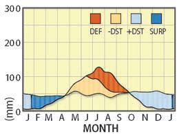
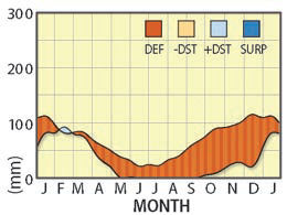
A water-balance diagram plots the average calculated water balance as a function of time, like this one for Madison, Wisconsin. Light orange depicts times of soil-water use, darker orange indicates times of deficit, light blue shows soil-water recharge, and darker blue depicts times of surplus. On the globes, a blue-green area would be considered a “wet” climate, whereas the orange and yellow areas would be considered to have a “dry” climate. This does not mean that the wet climate would be rainy all the time or that a dry climate might not have some precipitation.

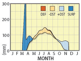
On the water-balance diagram, the two “DST” lines represent the estimated change in soil water from month to month (DST stands for “delta storage,” the change in the amount of stored water). A negative DST (light orange) indicates that conditions are drying out relative to the month before, and a positive DST (light blue) indicates that conditions are getting wetter. Note how positive and negative DSTs can precede a time of surplus or a time of deficit, respectively. This diagram for Madison, a Humid Continental climate, shows no climatological deficits and small surpluses, except when the spring thaw melts snow and ice, causing extremely high runoff totals. Precipitation mostly arrives when it is needed and typically doesn’t arrive in overwhelming amounts when it isn’t needed.

The very long, dry summer in Mediterranean climates, such as Los Angeles, causes large deficits during those months. Winter receives much more precipitation though, allowing for soil-water recharge from November into late winter and spring.

Montevideo, Uruguay, has a Humid Subtropical climate. Deficits are minimal even in the hot summer (which occurs in December through February) at this Southern Hemisphere location. Winter surpluses are kept relatively small by fairly high PE rates.

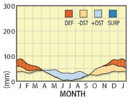
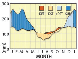
Tierra del Fuego is the cold, southernmost tip of South America (). It has soil-water use or deficits most of the year, except during the Southern Hemisphere winter (e.g., June and July).

The Marine West Coast climates of northwestern Europe, represented by Paris, have seasonal swings in water balance, with a small deficit typical during summer. Precipitation rarely occurs in huge deluges and soils have a high field capacity, so recharge requires a long time.

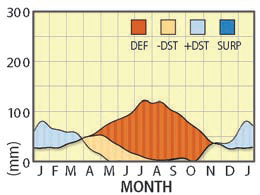
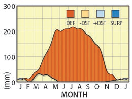
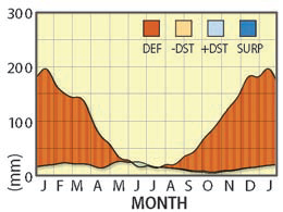
Desert climates like that at Riyadh, Saudi Arabia, show huge climatological deficits and little or no surplus. In this region, water is often brought in artificially.

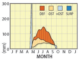
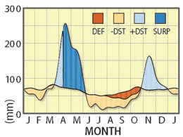
Subarctic climates like in Yakutsk, Russia, have odd water balance diagrams because there is no runoff during the long, frozen winter, but spring snowmelt gives extremely high runoff totals. Long summer daylight hours create some deficit values.

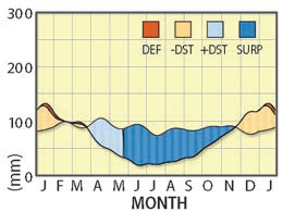
Tropical Rain Forest climates, like Port Moresby, Papua New Guinea, show long periods of abundant surplus and only short periods of very small deficits when the ITCZ moves farthest away. The warm temperatures and high rainfall amounts allow thick growths of rain-forest plants.

No climatological surpluses exist in the true desert climate of Windhoek, Namibia, but deficits are smaller than might be expected because a cold ocean current keeps temperatures (and therefore PE) somewhat suppressed.

Tropical Savanna climates, as in Nairobi and the central parts of Kenya, show double peaks in soil-water recharge, which correspond to times of year when the ITCZ makes its closest approach. Soil-water use and deficits occur when the subtropical high approaches.

Leonora, in the Australian Outback, has extremely high deficits, especially in the Southern Hemisphere summer. The lower temperatures, northward migration of the subtropical high, and occasional mid-latitude wave cyclone storminess in the Southern Hemisphere winter (June through August) permit a very brief period of soil-water recharge.